Conditional probability

In probability theory, the "conditional probability of $A$ given $B$ " is the probability of $A$ if $B$ is known to occur. It is commonly notated $P(A|B)$ , and sometimes $P_B(A)$ . (The vertical line should not be mistaken for logical OR.) $P(A|B)$ can be visualised as the probability of event $A$ when the sample space is restricted to event $B$ . Mathematically, it is defined for $\textstyle P(B) \ne 0$ as

$P(A|B) = \frac{P(A \cap B)}{P(B)}.$

Formally, $P(A|B)$ is defined as the probability of $A$ according to a new probability function on the sample space, such that outcomes not in $B$ have probability 0 and that it is consistent with all original probability measures. The above definition follows (see Formal derivation).^[1]

1 Definition
2 Example
3 Statistical independence
4 Common fallacies
- 4.1 Assuming conditional probability is of similar size to its inverse
- 4.2 Assuming marginal and conditional probabilities are of similar size
5 Formal derivation
6 See also
7 References
8 External links

Definition

Conditioning on an event

Given two events $A$ and $B$ in the same probability space with $P(B)>0$ , the conditional probability of $A$ given $B$ is defined as the quotient of the unconditional joint probability of $A$ and $B$ , and the unconditional probability of $B$ :

$P(A|B) \triangleq \frac{P(A \cap B)}{P(B)}$

The above definition is how conditional probabilities are introduced by Kolmogorov. However, other authors such as De Finetti prefer to introduce conditional probability as an axiom of probability. Although mathematically equivalent, this may be preferred philosophically; under major probability interpretations such as the subjective theory, conditional probability is considered a primitive entity. Further, this "multiplication axiom" introduces a symmetry with the summation axiom^[2]:

Multiplication axiom:

$P(A \cap B) = P(A|B)P(B)$

Summation axiom (A and B mutually exclusive):

$P(A \cup B) = P(A) %2B P(B)$

Definition with σ-algebra

If $P(B)=0$ , then the simple definition of $P(A|B)$ is undefined. However, it is possible to define a conditional probability with respect to a σ-algebra of such events (such as those arising from a continuous random variable).

For example, if X and Y are non-degenerate and jointly continuous random variables with density ƒ_X,Y(x, y) then, if B has positive measure,

$P(X \in A \mid Y \in B) = \frac{\int_{y\in B}\int_{x\in A} f_{X,Y}(x,y)\,dx\,dy}{\int_{y\in B}\int_{x\in\Omega} f_{X,Y}(x,y)\,dx\,dy} .$

The case where B has zero measure can only be dealt with directly in the case that B={y₀}, representing a single point, in which case

$P(X \in A \mid Y = y_0) = \frac{\int_{x\in A} f_{X,Y}(x,y_0)\,dx}{\int_{x\in\Omega} f_{X,Y}(x,y_0)\,dx} .$

If A has measure zero then the conditional probability is zero. An indication of why the more general case of zero measure cannot be dealt with in a similar way can be seen by noting that the limit, as all δy_i approach zero, of

$P(X \in A \mid Y \in \cup_i[y_i,y_i%2B\delta y_i]) \approxeq \frac{\sum_{i} \int_{x\in A} f_{X,Y}(x,y_i)\,dx\,\delta y_i}{\sum_{i}\int_{x\in\Omega} f_{X,Y}(x,y_i) \,dx\, \delta y_i} ,$

depends on their relationship as they approach zero. See conditional expectation for more information.

Conditioning on a random variable

Conditioning on an event may be generalized to conditioning on a random variable. Let $X$ be a random variable taking some value from $\{x_n\}$ . Let $A$ be an event. The probability of $A$ given $X$ is defined as

$P(A|X) = \begin{cases} P(A\mid X=x_0) & \text{if }X=x_0 \\ P(A\mid X=x_1) & \text{if }X=x_1 \\ \ldots \end{cases}$

Note that $P(A|X)$ and $X$ are now both random variables. From the law of total probability, the expected value of $P(A|X)$ is equal to the unconditional probability of $A$ .

Example

Consider the rolling of two fair six-sided dice.

Let $A$ be the value rolled on die 1
Let $B$ be the value rolled on die 2
Let $A_n$ be the event that $A=n$
Let $\Sigma_m$ be the event that $A%2BB \leq m$

Suppose we roll $A$ and $B$ . What is the probability that $A=2$ ? Table 1 shows the sample space. $A=2$ in 6 of the 36 outcomes, so $\textstyle P(A_2) = \frac{6}{36} = \frac{1}{6}$ .

Table 1
+	B=1	2	3	4	5	6
A=1	2	3	4	5	6	7
2	3	4	5	6	7	8
3	4	5	6	7	8	9
4	5	6	7	8	9	10
5	6	7	8	9	10	11
6	7	8	9	10	11	12

Suppose however that somebody else rolls the dice in secret, revealing only that $A%2BB \le 5$ . Table 2 shows that $A%2BB \le 5$ for 10 outcomes. $A=2$ in 3 of these. The probability that $A=2$ given that $A%2BB \leq 5$ is therefore $\textstyle \frac{3}{10} = 0.3$ . This is a conditional probability, because it has a condition that limits the sample space. In more compact notation, $P(A_2 | \Sigma_5) = 0.3$ .

Table 2
+	B=1	2	3	4	5	6
A=1	2	3	4	5	6	7
2	3	4	5	6	7	8
3	4	5	6	7	8	9
4	5	6	7	8	9	10
5	6	7	8	9	10	11
6	7	8	9	10	11	12

Statistical independence

If two events $A$ and $B$ are statistically independent, the occurrence of $A$ does not affect the probability of $B$ , and vice versa. That is,

$P(A|B) \ = \ P(A)$

$P(B|A) \ = \ P(B)$ .

Using the definition of conditional probability, it follows from either formula that

$P(A \cap B) \ = \ P(A) P(B)$

This is the definition of statistical independence. This form is the preferred definition, as it is symmetrical in $A$ and $B$ , and no values are undefined if $P(A)$ or $P(B)$ is 0.

Common fallacies

Assuming conditional probability is of similar size to its inverse

Main article: Confusion of the inverse

In general, it cannot be assumed that $P(A|B) \approx P(B|A)$ . This can be an insidious error, even for those who are highly conversant with statistics.^[3] The relationship between $P(A|B)$ and $P(B|A)$ is given by Bayes' theorem:

$P(B|A) = P(A|B) \frac{P(B)}{P(A)}.$

That is, $P(A|B) \approx P(B|A)$ only if $\textstyle \frac{P(B)}{P(A)}\approx 1$ , or equivalently, $\textstyle P(A)\approx P(B)$ .

Assuming marginal and conditional probabilities are of similar size

In general, it cannot be assumed that $P(A) \approx P(A|B)$ . These probabilities are linked through the formula for total probability:

$P(A) \, = \, \sum_n P(A \cap B_n) \, = \, \sum_n P(A|B_n)P(B_n)$ .

This fallacy may arise through selection bias.^[4] For example, in the context of a medical claim, let $S_C$ be the event that sequelae $S$ occurs as a consequence of circumstance $C$ . Let $H$ be the event that an individual seeks medical help. Suppose that in most cases, $C$ does not cause $S$ so $P(S_C)$ is low. Suppose also that medical attention is only sought if $S$ has occurred. From experience of patients, a doctor may therefore erroneously conclude that $P(S_C)$ is high. The actual probability observed by the doctor is $P(S_C|H)$ .

Formal derivation

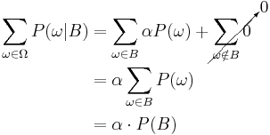
This section is based on the derivation given in Grinsted and Snell's Introduction to Probability.^[5]

Let $\Omega$ be a sample space with elementary events $\{\omega\}$ . Suppose we are told the event $B \subseteq \Omega$ has occurred. A new probability distribution (denoted by the conditional notation) is to be assigned on $\{\omega\}$ to reflect this. For events in $B$ , It is reasonable to assume that the relative magnitudes of the probabilities will be preserved. For some constant scale factor $\alpha$ , the new distribution will therefore satisfy:

$\text{1. }\omega \in B�: P(\omega|B) = \alpha P(\omega)$

$\text{2. }\omega \notin B�: P(\omega|B) = 0$

$\text{3. }\sum_{\omega \in \Omega} {P(\omega|B)} = 1.$

Substituting 1 and 2 into 3 to select $\alpha$ :

$\begin{align} \sum_{\omega \in \Omega} {P(\omega | B)} &= \sum_{\omega \in B} {\alpha P(\omega)} %2B \cancelto{0}{\sum_{\omega \notin B} 0} \\ &= \alpha \sum_{\omega \in B} {P(\omega)} \\ &= \alpha \cdot P(B) \\ \end{align}$

$\implies \alpha = \frac{1}{P(B)}$

So the new probability distribution is

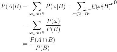
$\text{1. }\omega \in B�: P(\omega|B) = \frac{P(\omega)}{P(B)}$

$\text{2. }\omega \notin B�: P(\omega| B) = 0$

Now for a general event $A$ ,

$\begin{align} P(A|B) &= \sum_{\omega \in A \cap B} {P(\omega | B)} %2B \cancelto{0}{\sum_{\omega \in A \cap B^c} P(\omega|B)} \\ &= \sum_{\omega \in A \cap B} {\frac{P(\omega)}{P(B)}} \\ &= \frac{P(A \cap B)}{P(B)} \end{align}$

References

^ George Casella and Roger L. Berger (1990), Statistical Inference, Duxbury Press, ISBN 0534119581 (p. 18 et seq.)
^ Gillies, Donald (2000); "Philosophical Theories of Probability"; Routledge; Chapter 4 "The subjective theory"
^ Paulos, J.A. (1988) Innumeracy: Mathematical Illiteracy and its Consequences, Hill and Wang. ISBN 0809074478 (p. 63 et seq.)
^ Thomas Bruss, F; Der Wyatt Earp Effekt; Spektrum der Wissenschaft; March 2007
^ Grinstead and Snell's Introduction to Probability, p. 134

External links

Weisstein, Eric W., "Conditional Probability" from MathWorld.
F. Thomas Bruss Der Wyatt-Earp-Effekt oder die betörende Macht kleiner Wahrscheinlichkeiten (in German), Spektrum der Wissenschaft (German Edition of Scientific American), Vol 2, 110–113, (2007).
Conditional Probablity Problems with Solutions